Staying Alive: Uncensored Survival Analysis with Tabular Foundation Models
In the last couple of years we’ve witnessed how Tabular Foundation Models (TFMs) became an exciting major research direction, showing how the foundation model paradigm extends beyond LLMs. TFMs have proven useful for a variety of tasks and domains, and have shown impressive results across numerous benchmarks when used out-of-the-box. Now, not all predictive tasks can be addressed with an off-the-shelf TFM, and in this blog post we’re going to explore a particular case: Survival Analysis.
Survival Analysis (SA) is a statistical framework that aims at modeling the time span until some event of interest takes place. This type of data is usually referred to as time-to-event data. For example, one might be interested in observing the survival outcomes of patients that participate in a clinical trial, or in predicting whether a user will discontinue a streaming service. In general, the practitioner establishes a time window for running the analysis and, as a result, the time of the event is not observed for some subjects just because the event of interest didn’t take place within that time period. This phenomenon is called right censoring and it can be deemed the SA equivalent of missing data.
Right censoring is actually a very hard problem and classical imputation mechanisms are not directly applicable. Say you’re analyzing the survival outcome of patients that were involved in a clinical trial. Some patients might drop early from the study because they decided to no longer take part in it. For those patients you can observe their time of censoring. But for those patients who survived beyond the time when the study finished, there’s no information whatsoever about when death occurred — one can safely assume such “event” will take place eventually for everyone. Classical SA frameworks such as Cox models and Accelerated Failure Time (AFT) models can directly account for this phenomenon in the formulation of their parameter fitting problem. But remember that we want to use TFMs — whose parameters are frozen, so how can we incorporate information from these censored subjects? In other words, how can we reformulate SA with censored data as a purely predictive task, without having to train a survival model from scratch?
That’s precisely what we do in this blog. After introducing some basics, we will show how to use a TFM to build an AFT model with no training except for the fitting of a single scalar parameter. We’ll argue that naively disregarding censored data — the Complete Case Analysis (CCA) — biases the model towards underestimating survival times, leaving a lot of headroom for improvement. And finally, the most interesting part, we’ll see how we can leverage TFMs to impute censored data through an in-context iterative estimator. This is a great example of how one can iteratively refine the context of the TFM to boost performance. Interestingly, we’ll see how the performance of the model improves throughout iterations.
Some SA background
A typical time-to-event dataset has the form \{(t_i, \Delta_i, \mathbf{x}_i)\}_{i=1}^N, where \mathbf{x}_iis a feature vector, t_i = \min(T_i, C_i)is the observed time, T_iis the event time, C_iis the censoring time and \Delta_i = \mathbf{1}(\tilde{t}_i \leq C_i)indicates whether the event was observed for subject i. In other words, if \Delta_i = 0then subject iis censored. In this blog we consider the scenario where the censoring time is constant and corresponds to the time the study finished.
A crucial quantity that SA aims at modelling is the survival function defined as S(t|\mathbf{x}) = p(T>t|\mathbf{x}). This function represents the probability of an observation with features \mathbf{x}surviving past time t. In our clinical trial example from before, the survival function of a patient with some specific biomarker values tells us about their chances of surviving past some number of weeks following a treatment. S(t|x)can have different forms depending on the choice of the model. In this blog we choose the Accelerated Failure Time (AFT) model, which linearly regresses the logarithm of the event time as
where \epsilon_i \overset{\text{i.i.d.}}{\sim} \mathcal{N}(0,1). Denoting \mu_i = \mathbf{x}_i^\top \beta, the corresponding survival function is
where \Phidenotes the standard Gaussian cumulative distribution function.
Under right censoring, the log-likelihood is given by
Note that this quantity is a function of the scalar parameter \sigma, and it can be fit very efficiently with a scipy.optimize function. This detail will be important in a bit.
The Buckley-James estimator
At this point it’s important to notice that there are sophisticated mechanisms to impute censored data for SA. A prominent example is the Buckley-James (BJ) estimator. Because this work is very much inspired by this method here’s a short overview of how it works.
The BJ estimator replaces each censored outcome with its expected value given that the true event time exceeds the censoring time, and it estimates this value non-parametrically from the model’s own residuals via Kaplan-Meier. One can then refit the regression on this “complete” dataset, recompute the imputations, and repeat until values stabilize. At each iteration, it defines the targets as follows:
where \tilde{e}_i = \log t_i - \hat{\mu}_iis the observed residual, \hat{F}_\epsilonis the Kaplan-Meier estimate of the residual distribution fitted on \{(\tilde{e}_i, \Delta_i)\}_{i=1}^N, and w_jare the probability masses assigned by \hat{F}_\epsilonat each uncensored residual.
If you’re thinking that this resembles a lot an EM loop, you’re right: one imputes the missing outcomes with the model’s current knowledge, then refit the model, and repeat. In other words, the Buckley-James procedure iteratively solves the following fixed point equation:
This blog is all about replacing the ordinary least square (OLS) regression step from BJ with an In-Context TFM, while keeping the imputation loop.
Doing SA with TFMs
Let (X_{\text{tr}}, \mathbf{t}_{\text{tr}}, \mathbf{\Delta}_{\text{tr}})denote the training set and X_{\text{test}}the test set. Let’s also define \mathcal{U} = \{i : \Delta_i = 1\}and \mathcal{C} = \{i : \Delta_i = 0\}as the set of uncensored and censored training instances respectively. Finally, let fdenote a TFM used as a regressor backbone.
One can leverage a TFM to build a survival model as follows. First, we estimate \mu,
and then estimate \sigmaby maximizing the log-likelihood defined above:
over the full training set. Note that \sigmais a single scalar parameter. Once obtained, we can define a time grid, say, t = 1, 2, 3, \dotsand use the formula for S(t|\mathbf{x})defined above to obtain survival curves. The problem with naively disregarding censored observations is that this biases the model towards underestimating survival times. The thing is that censored data carries important information that needs to be incorporated into the model. That’s precisely what we’re going to introduce next: a BJ-inspired in-context estimator for imputing censored data.
Imputing censored data with TFMs
Let’s now address the main question of this blog, how can we leverage TFMs to impute censored data and provide SA with a “complete” dataset? Classical SA algorithms naturally account for censored data by incorporating censored information into their parameter estimation formulation. But in our case, the TFM weights are frozen, and, as a result, we need to account for censored data while framing survival regression as a purely in-context prediction task.
Luckily for us this is perfectly possible. The core idea is to use a TFM as a non-parametric in-context estimator to iteratively impute survival times as pseudo-targets. Pseudo-targets are initialized with a data-driven warm start based on the Kaplan-Meier jackknife estimator. Then, similar to the BJ procedure, we alternate between refining the pseudo-targets and updating the scale parameter \sigma.
Let’s explore these stages one by one.
Initialization
Let t_0be the median observed event time and \tilde{\theta}_ithe jackknife pseudo-observation of subject iat t_0, obtained via leave-one-out Kaplan-Meier estimation. We initialize \hat{\sigma}^{(0)}by maximizing its NLL defined in the previous section using pseudo-observation-based predictions. Censored pseudo-targets are then initialized as:
for i \in \mathcal{C}. This formulation inverts the AFT survival function at t_0to map pseudo-targets on the survival probability scale back to imputed log-times. The \maxoperation enforces T_i > C_i, that is, that the event for censored data takes place after the censoring time.
Pseudo-targets and scale updates at iteration k
At each iteration k, we form a context \mathcal{U}^{(k)}\cup\mathcal{C}^{(k)}, with \mathcal{U}^{(k)} \subseteq \mathcal{U}and \mathcal{C}^{(k)} \subseteq \mathcal{C}, by sub-sampling censored and uncensored subjects from the training set. This ensures that each censored subject is predicted out-of-sample, preventing degenerate self-prediction. Then we use a TFM to predict the mean log-time of the remaining censored subjects:
With that, we can update the pseudo-targets as follows:
where \epsilon_i^{(k)} \overset{\text{i.i.d.}}{\sim} \mathcal{N}(0,1). Note that our updates are drawn from a truncated distribution p(\log T_i| T_i > C_i; \hat{\mu}_i^{(k)}, \hat{\sigma}^{(k-1)})that enforces the constraint that T_i > C_ifor censored subjects. Finally, we can fit \sigmaby MLE on the full training set, comprising both censored and uncensored subjects:
We repeat this procedure until the targets stabilize or a maximum number of iterations is reached.
Inference
Here’s the final piece of the puzzle. At test time, we just make a forward pass with the TFM using the “complete”, imputed dataset obtained from our iterative procedure:
where Kis the last iteration, and calculate the survival function on a predefined time grid using \sigma = \sigma^{(K)}.
Experiments
We benchmark our method against classical survival models on five publicly available datasets, using both TabPFN and TabICL as backbones.
Datasets
| Dataset | Samples | Features | Censoring |
|---|---|---|---|
| WHAS500 | 500 | 14 | 57.0% |
| GBSG | 686 | 8 | 56.4% |
| METABRIC | 1,904 | 9 | 42.0% |
| SUPPORT | 8,873 | 14 | 31.9% |
| FLCHAIN | 7,874 | 9 | 72.5% |
These span cardiovascular disease (WHAS500), breast cancer (GBSG, METABRIC), critical care (SUPPORT), and a serum biomarker study (FLCHAIN). All continuous variables are standardized; results are reported over 10 random 80/20 train-test splits.
Setup
Baselines are four classical models fitted from scratch on each split: Cox PH, Weibull AFT, Log-Normal AFT, and Random Survival Forest (RSF). We also compare against TabSA-Bin (Kim et al.) as the main zero-shot competitor. It reframes survival analysis as binary classification over Kevent-time quantile bins, assembling a step-function survival curve from TFM predictions. It’s effective, but discretizing time introduces a resolution–context tradeoff that our method sidesteps by operating in continuous time.
Our method (TabSA) comes in three flavors:
- TabSA-CCA: complete case analysis — regress log-time of uncensored subjects only.
- TabSA-PO: KM jackknife pseudo-observations as imputed targets before regression.
- TabSA-BJ: iterative Buckley-James-inspired imputation, alternating between refining censored pseudo-times and re-estimating \sigmaover 10 iterations, with 50% censored subsampling at each step.
Metrics: Harrell’s C-index (\uparrow) and IPCW Integrated Brier Score (IBS, \downarrow), integrated from the 5th to 95th percentile of observed training times. Bold = significantly better (paired t-test, \alpha = 0.05); underline = best zero-shot method per column.
Results
Results are summarized in the following table.
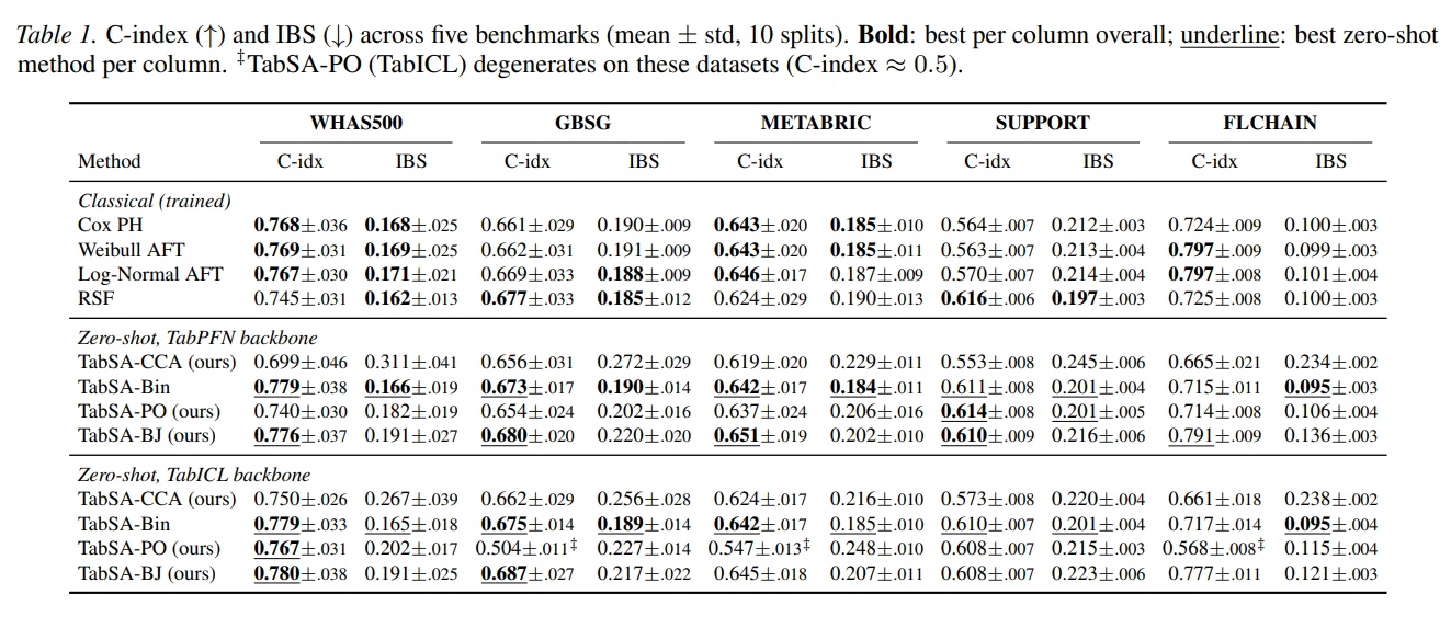
TabSA-BJ improves over its simpler variants on C-index, with the largest gains on high-censoring datasets. On IBS, all continuous-time TabSA variants fall behind TabSA-Bin — discretization appears to help calibration. This makes sense: TabSA-Bin directly predicts survival probabilities at fixed quantiles, which naturally suits calibration. Our method operates in log-time space, preserving rank structure and driving higher C-index. The two are complementary rather than competing. Classical methods remain strong on IBS, but our method often matches or beats them on discrimination — with no dataset-specific training. TabICL and TabPFN perform comparably overall, though TabICL yields degenerate results for TabSA-PO on three datasets.
Convergence
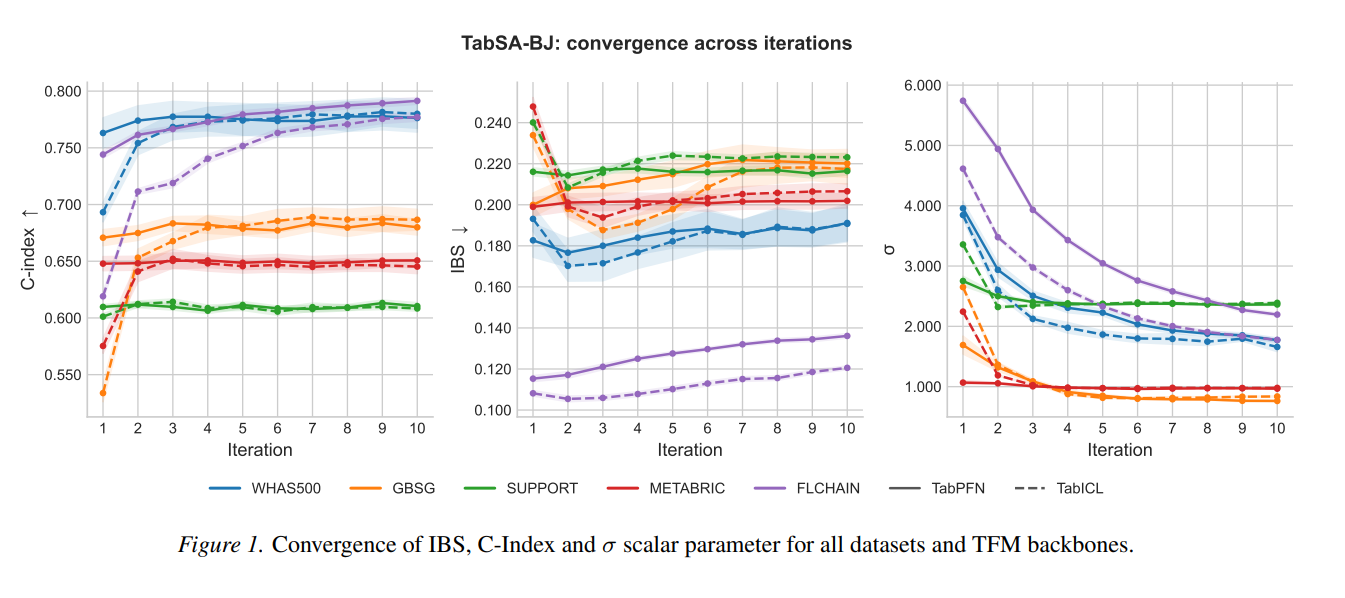
The following plot shows how \sigmaconverges, and how the IBS and CI metrics stabilize.
This figure is interesting for two reasons. First, \sigmaconverges to a stable value across iterations, confirming that the pseudo-targets reach a fixed point. On several datasets \sigmaapproaches 1, suggesting the TFM captures a meaningful fraction of log-time variance under the AFT model — without ever being trained on survival data.
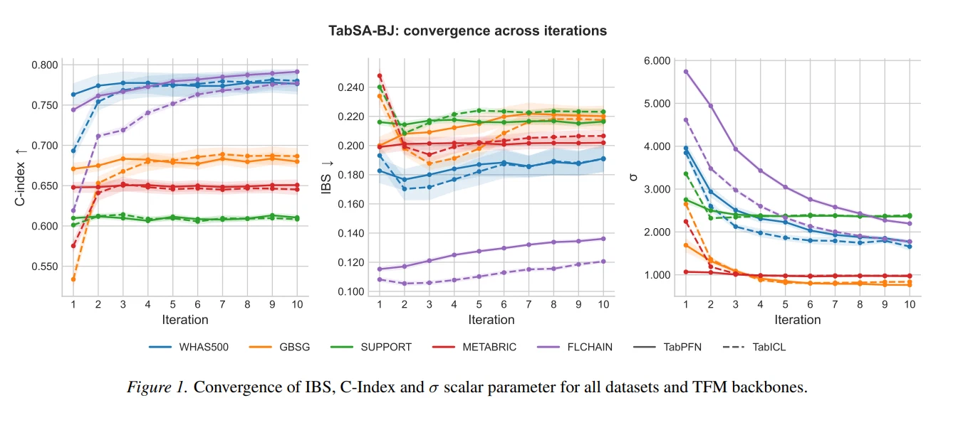
The second reason has to do with the context-engineering angle of this experiment. Note that the performance tends to increase with iterations, sometimes peaking as \sigmastabilizes, like the C-index, or reaching the best score after a couple of iterations, like IBS. This not only suggests that the number of iterations can be finetuned (especially for IBS, that tends to get worse at later iterations), but also that one can benefit from iteratively refining the context that’s fed to the TFM.
Conclusion
In this blog we introduced a TFM-based mechanism requiring no dataset-specific training – beyond fitting a single scalar parameter — for doing zero-shot survival regression. We also showed how to leverage TFMs for iteratively imputing censored data and provide the survival algorithm with a “complete” dataset. The full workshop paper is in Arxiv, and the code is here.